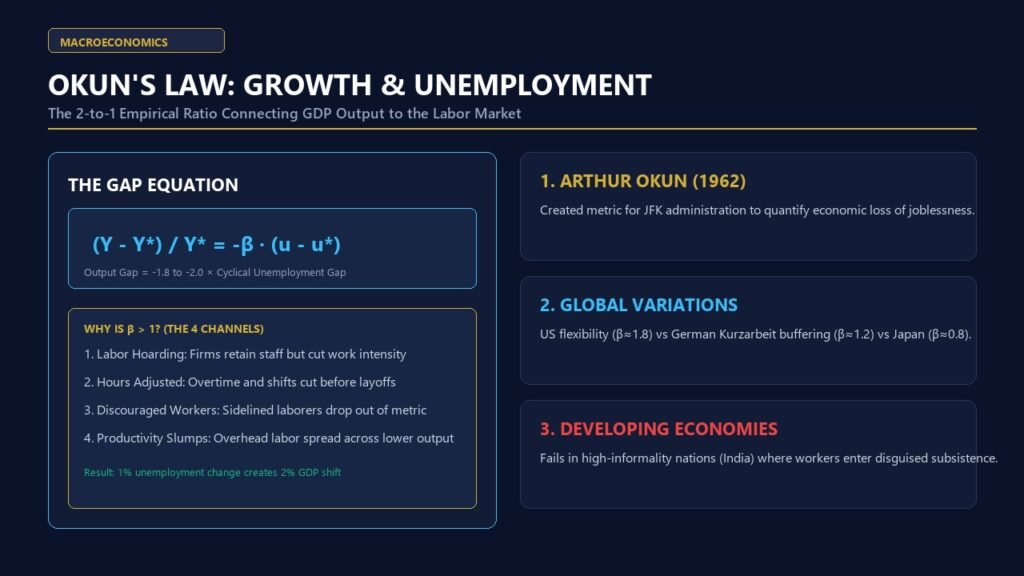
Executive Definition: Okun’s law explained simply is an empirically observed macroeconomic rule of thumb describing the stable, inverse relationship between a country’s economic output growth and changes in its unemployment rate. Formulated in 1962 by American economist Arthur Okun, the law posits that for every 1 percentage point increase in the unemployment rate above its natural rate, an economy’s real Gross Domestic Product (GDP) contracts by approximately 2 percentage points below its potential output.
In central banking and fiscal planning, policymakers cannot calibrate stimulus or monetary tightening without a reliable gauge of spare productive capacity. While headline Gross Domestic Product measures overall transactional volume, it reveals little about whether factories are lying idle or whether millions of willing workers are sidelined from productive employment. Having Okun’s law explained through its mathematical formulations, labor-market friction channels, and modern empirical breakdowns provides institutional analysts and economics students with the quantitative bridge connecting national output to the labor market.
Table of Contents
- 1. Historical Origins: Arthur Okun and the Kennedy Council of Economic Advisers
- 2. Mathematical Specifications: The Gap Version vs. The Difference Version
- 3. Why the Okun Coefficient Exceeds 1: The Four Microeconomic Transmission Channels
- 4. Step-by-Step Worked Numerical Example: Estimating the Output Gap
- 5. Cross-Country Variations: US Flexibility vs. European Sclerosis vs. Asian Models
- 6. Post-Crisis Breakdowns: Jobless Recoveries and Remote Work Dynamics
- 7. Okun’s Law in Developing Economies: India’s Informal Labor Reality
- 8. Comparative Matrix: Okun Coefficients Across Major Global Economies
- 9. Frequently Asked Questions (FAQ)
- 10. Authoritative References & Primary Sources
1. Historical Origins: Arthur Okun and the Kennedy Council of Economic Advisers
In 1962, Yale professor Arthur Okun was serving as a senior staff economist on President John F. Kennedy’s Council of Economic Advisers (later serving as its Chairman under Lyndon B. Johnson). The Kennedy administration was attempting to convince Congress to pass a landmark tax cut to stimulate sluggish economic growth. To justify fiscal intervention, Okun needed an objective, defensible metric to quantify the economic loss resulting from unemployment.
In his seminal paper, “Potential GNP: Its Measurement and Significance,” published in the Proceedings of the American Statistical Association, Okun analyzed quarterly United States time-series data from 1947 to 1960. He uncovered a remarkably robust statistical regularity: every 1 percentage point drop in the national unemployment rate was associated with approximately a 3% expansion in real Gross National Product (GNP). In subsequent decades, as labor market structures evolved, modern econometric revisions adjusted this historical 3-to-1 ratio toward a contemporary 2-to-1 benchmark.
2. Mathematical Specifications: The Gap Version vs. The Difference Version
In contemporary macroeconomics, Okun’s Law is formally estimated using two complementary mathematical representations:
\text{The Gap Version: } \frac{Y – Y^*}{Y^*} = -\beta (u – u^*)
Where:
- $Y$ is actual real Gross Domestic Product.
- $Y^*$ is potential GDP (the sustainable level of output achievable when capital and labor operate at normal full-capacity utilization).
- $\frac{Y – Y^*}{Y^*}$ is the percentage output gap.
- $u$ is the actual civilian unemployment rate.
- $u^*$ is the natural rate of unemployment (or NAIRU — Non-Accelerating Inflation Rate of Unemployment).
- $\beta$ is the Okun coefficient (empirically estimated between $1.5$ and $2.0$ for the United States).
The second specification, widely favored by financial market analysts who lack unobservable estimates of potential output, is the Difference (or Growth Rate) Version:
\Delta u_t = -\alpha (g_t – g^*)
Where $\Delta u_t = u_t – u_{t-1}$ is the year-over-year change in the unemployment rate, $g_t$ is the actual annual real GDP growth rate, $g^*$ is the economy’s long-run potential GDP growth rate (typically around 2.0% in advanced economies), and $\alpha \approx 0.5$ is the responsiveness coefficient. If real GDP grows at its potential rate ($g_t = g^*$), the unemployment rate remains constant ($\Delta u_t = 0$). For unemployment to fall by 1 percentage point over a year, real GDP must grow at $g^* + \frac{1}{\alpha} = 2.0\% + 2.0\% = 4.0\%$.
3. Why the Okun Coefficient Exceeds 1: The Four Microeconomic Transmission Channels
A naive intuition suggests that if employment drops by 1%, output should drop by roughly 1% (assuming labor contributes approximately two-thirds of national income). Why then does a 1 percentage point shift in unemployment correspond to an outsized 2% change in GDP? The answer lies in four interrelated microeconomic labor market channels:
- 1. Labor Hoarding by Employers: Terminating employees during a downturn and rehiring new personnel during a recovery imposes massive institutional costs (severance packages, advertising, interviewing, background checks, and training). Consequently, when demand softens, firms retain trained employees but reduce their work intensity. Factory workers might spend hours maintaining machinery rather than assembling goods. Thus, measured unemployment rises slowly, but output drops sharply.
- 2. Variation in Average Work Hours: Before initiating layoffs, employers systematically cut overtime hours, eliminate weekend shifts, or reduce work schedules from 40 hours to 32 hours per week. A substantial drop in total labor hours occurs without appearing as an increase in the headline U-3 unemployment rate.
- 3. The Discouraged Worker Effect (Labor Force Participation): The official unemployment rate measures only active job-seekers ($u = \frac{\text{Unemployed}}{\text{Labor Force}}$). During severe contractions, hundreds of thousands of frustrated workers stop actively seeking jobs, dropping out of the labor force entirely. Because they are no longer counted as unemployed, the official unemployment rate understates the true destruction of productive capacity.
- 4. Procyclical Labor Productivity: In modern economies, fixed overhead labor (management, accounting, legal compliance, IT security) must be maintained regardless of whether sales volume is high or low. When output drops, these fixed labor costs are spread across fewer units of product, causing output per worker to collapse procyclically.
4. Step-by-Step Worked Numerical Example: Estimating the Output Gap
Consider an advanced economy with the following macroeconomic data observed by its central bank:
- Current Actual Real GDP ($Y$): $\$24.0$ trillion.
- Current Actual Unemployment Rate ($u$): $6.5\%$.
- Central Bank Estimate of Natural Rate of Unemployment ($u^*$): $4.5\%$.
- Empirical Okun Coefficient ($\beta$): $1.80$.
Step 1: Calculate the Unemployment Gap
\text{Unemployment Gap} = u – u^* = 6.5\% – 4.5\% = +2.0\%
Step 2: Calculate the Percentage Output Gap using Okun’s Law
\text{Output Gap} = -\beta \cdot (u – u^*) = -1.80 \times (+2.0\%) = -3.60\%
The national economy is operating 3.60% below its potential capacity.
Step 3: Solve for Potential GDP ($Y^*$) and Absolute Lost Output
\frac{Y – Y^*}{Y^*} = -0.036 \implies Y = Y^*(1 – 0.036) = 0.964 Y^*
Y^* = \frac{\$24.0 \text{ trillion}}{0.964} \approx \$24.896 \text{ trillion}
\text{Lost Annual Output} = Y^* – Y = \$24.896 \text{ T} – \$24.000 \text{ T} = \$896 \text{ billion}
The 2.0% excess unemployment rate deprives the economy of nearly $900 billion in lost goods and services every year.
5. Cross-Country Variations: US Flexibility vs. European Sclerosis vs. Asian Models
The magnitude of the Okun coefficient varies significantly across global jurisdictions due to structural differences in labor market institutions:
- United States ($\beta \approx 1.8 – 2.0$ — High Cyclical Sensitivity): Operating under an “employment-at-will” legal framework with relatively low severance requirements and minimal union coverage in the private sector, American corporations adjust headcounts rapidly during recessions. Unemployment surges quickly during downturns and falls briskly during expansions.
- Germany & France ($\beta \approx 1.1 – 1.4$ — Institutional Buffering): European economies feature stringent Employment Protection Legislation (EPL), mandatory severance consultations, and government-subsidized short-time work schemes (such as Germany’s famous Kurzarbeit). During recessions, German employers preserve jobs while the state subsidizes reduced hours. As a result, unemployment barely fluctuates, dampening the Okun coefficient.
- Japan ($\beta \approx 0.8 – 1.0$ — Lifetime Employment Norms): Rooted in traditional corporate cultural norms of long-term job security, major Japanese conglomerates absorb demand contractions by compressing executive compensation and shifting workers across subsidiary divisions rather than executing mass layoffs.
6. Post-Crisis Breakdowns: Jobless Recoveries and Remote Work Dynamics
While Okun’s Law remains an indispensable conceptual tool, its stability has faced significant challenges in recent business cycles:
- The Era of “Jobless Recoveries” (1991, 2001, 2008): Following late-20th and early-21st-century recessions, GDP growth rebounded swiftly, but employment remained depressed for multiple years. Corporations leveraged digital automation and global outsourcing to expand output without recalling laid-off domestic workers.
- The Post-Pandemic Labor Hoarding Paradox (2022–2024): Following the chaotic labor shortages of 2021, corporate executives became terrified of firing staff even when central banks launched aggressive interest rate hiking cycles. GDP growth decelerated, but unemployment remained near historic lows (3.5%–4.0%), leading to a temporary decoupling of Okun’s law.
7. Okun’s Law in Developing Economies: India’s Informal Labor Reality
Applying Okun’s Law to emerging economies like India reveals severe structural limitations. Over 80% of India’s workforce operates within the informal economy (agricultural labor, construction day-laborers, and small street enterprises) without formal contracts or unemployment insurance.
In such an environment, poor workers cannot afford to remain openly “unemployed” (they cannot survive without daily income). When an economic shock hits, workers do not register as unemployed; rather, they transition into disguised unemployment—returning to subsistence farming in ancestral villages or taking low-productivity gig jobs. Consequently, official Indian headline unemployment figures remain artificially low and unresponsive to large swings in GDP growth.
To examine how central banks incorporate output and employment gaps into policy interest rate rules, see our comprehensive guide on the Taylor Rule for central banks and review how wage pressures feed into price changes in our analysis of the Phillips Curve.
8. Comparative Matrix: Okun Coefficients Across Major Global Economies
| Country | Typical Okun Coefficient ($\beta$) | Labor Market Rigidity | Primary Adjustment Mechanism |
|---|---|---|---|
| United States | $1.8 – 2.0$ | Low (At-will employment) | Rapid headcount layoffs and rehiring |
| United Kingdom | $1.5 – 1.7$ | Moderate | Mixed: layoffs and flexible wage contracts |
| Germany | $1.1 – 1.3$ | High (Strong collective bargaining) | Working hours adjustments (Kurzarbeit) |
| Japan | $0.8 – 1.0$ | High (Cultural job protection) | Bonus cuts, internal transfers, productivity shifts |
| India | Weak / Statistically Unstable | Dualistic (Strict formal, vast informal) | Migration into informal and agricultural sectors |
9. Frequently Asked Questions (FAQ)
What is Okun’s Law in simple terms?
Okun’s Law states that when economic growth is strong, unemployment falls, and when economic growth is weak or negative, unemployment rises. Specifically, it suggests that a 1 percentage point increase in unemployment corresponds to roughly a 2% drop in GDP below its potential.
Is Okun’s Law a rigid physical law of nature?
No. Okun’s Law is an empirical rule of thumb based on historical statistical observation, not an unchangeable scientific law. Its coefficient shifts over time depending on labor market regulations, technology adoption, and demographics.
Why is the Okun coefficient usually around 2 instead of 1?
Because when companies experience declining demand, they do not merely fire workers. They also cut overtime, reduce workweek hours, suffer productivity drops, and some workers exit the labor force altogether. All these factors amplify the output drop relative to measured unemployment.
How do central banks use Okun’s Law?
Central banks use Okun’s Law to estimate the unobservable “output gap” from observable unemployment data. If actual unemployment is far above the natural rate, the central bank knows the economy is operating below capacity and may cut interest rates to stimulate activity.
Why does Okun’s Law work poorly in developing countries like India?
Because developing economies have large informal sectors where workers cannot afford to be unemployed. When the economy slows down, workers take informal or subsistence jobs rather than registering as unemployed, masking the true economic impact in official statistics.
10. Authoritative References & Primary Sources
- Okun, Arthur M. (1962). “Potential GNP: Its Measurement and Significance.” Proceedings of the Business and Economic Statistics Section of the American Statistical Association, 98–104.
- Ball, Laurence, Leigh, Daniel, & Loungani, Prakash. (2017). “Okun’s Law: Fit at 50?” Journal of Money, Credit and Banking, 49(7), 1413–1441.
- Knotek, Edward S., II. (2007). “How Useful Is Okun’s Law?” Federal Reserve Bank of Kansas City Economic Review, Q4, 73–103.
- International Monetary Fund (IMF). (2019). “Okun’s Law in Advanced and Emerging Economies: A Comprehensive Reassessment.” IMF Working Papers.
- Bureau of Labor Statistics (BLS). (2024). “Labor Force Statistics from the Current Population Survey.” BLS Official Portal.