Introduction to Inflationary Mechanics
Inflation is not a monolithic phenomenon. To prescribe the correct macroeconomic policy, economists must diagnose whether rising prices are caused by an excess of aggregate demand or a constriction of aggregate supply. The Aggregate Demand-Aggregate Supply (AD-AS) model is the standard diagnostic framework.
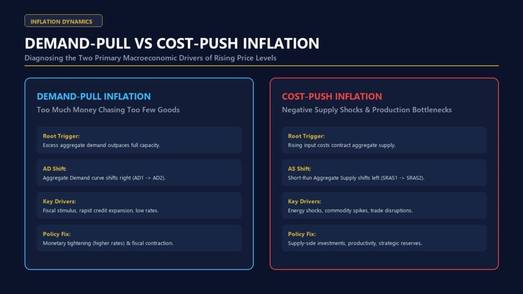
Demand-Pull Inflation: “Too much money chasing too few goods”
Demand-pull inflation occurs when aggregate demand (AD) shifts to the right, surpassing the economy’s potential output (Long-Run Aggregate Supply, LRAS).
Causes include expansionary fiscal policy (stimulus checks, deficit spending), loose monetary policy (low interest rates), or export booms. In the AD-AS model, the rightward shift of AD causes both the price level ($P$) and output ($Y$) to rise in the short run.
Cost-Push Inflation: Supply Shocks
Cost-push inflation occurs when Short-Run Aggregate Supply (SRAS) shifts to the left due to an increase in the costs of production independent of aggregate demand.
Causes include spikes in commodity prices (e.g., oil), supply chain disruptions, or aggressive wage increases unlinked to productivity. The leftward shift of SRAS results in a higher price level ($P$) but lower output ($Y$). This toxic combination is known as Stagflation.
Worked Numerical Example: The Quantity Theory of Money
Monetarists explain demand-pull inflation using the Equation of Exchange: $$ M \cdot V = P \cdot Y $$
Where M = Money Supply, V = Velocity of Money, P = Price Level, Y = Real GDP.
Assume an economy is at full employment ($Y$ is fixed at 100). The money supply ($M$) is $500, and Velocity ($V$) is 2. The Price Level ($P$) is: $$ P = \frac{M \cdot V}{Y} = \frac{500 \cdot 2}{100} = 10 $$
If the central bank aggressively expands the money supply to $600 while $Y$ and $V$ remain constant, the new price level becomes: $$ P = \frac{600 \cdot 2}{100} = 12 $$
Prices have risen by 20%. This is pure demand-pull inflation driven by monetary expansion.
Real-World Case Study: The 1970s Oil Crisis (Cost-Push)
In 1973, OPEC imposed an oil embargo, quadrupling the price of oil. Because oil is a primary input for almost all goods and transportation, the global SRAS curve shifted violently to the left. The US experienced stagflation: inflation reached double digits while unemployment surged. Central banks faced a dilemma: raising interest rates to fight inflation would worsen unemployment, but lowering rates to help employment would worsen inflation.
Frequently Asked Questions
How do central banks respond to Demand-Pull inflation?
Central banks respond aggressively to demand-pull inflation by raising interest rates. This cools down borrowing, investment, and consumption, shifting the AD curve back to the left to align with potential output.
Why is Cost-Push inflation harder for central banks to fix?
Central banks control demand (via interest rates), not supply. They cannot drill more oil or fix shipping delays. If they raise rates to stop cost-push inflation, they deepen the recession. If they lower rates to boost output, they risk hyperinflation. They usually have to “look through” temporary supply shocks and hope they resolve themselves.