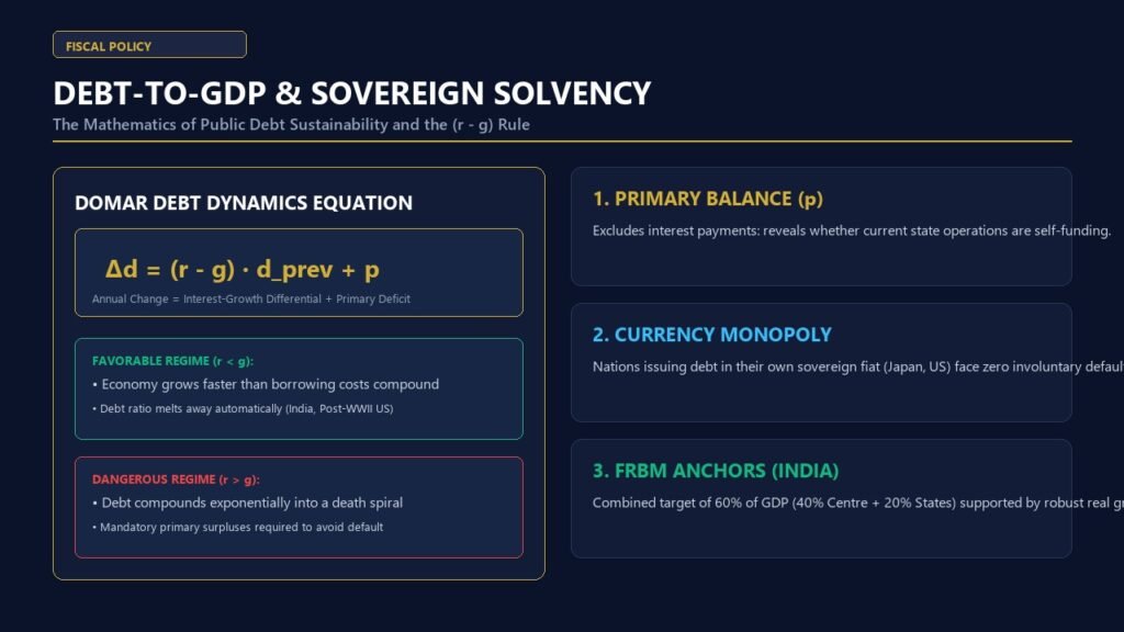
Executive Definition: The debt to GDP ratio explained simply is the fundamental metric of sovereign fiscal health comparing a nation’s cumulative gross public debt liabilities to its annual Gross Domestic Product. Expressed as a percentage, it measures a country’s leverage and capacity to service its sovereign obligations without defaulting or resorting to hyperinflationary currency debasement. A sustainable debt trajectory depends not merely on the static headline ratio, but on the dynamic relationship between sovereign borrowing costs ($r$) and the nominal economic growth rate ($g$).
In the wake of global crises, unprecedented peacetime pandemic spending, and demographic aging, global public debt has crossed $100 trillion, pushing sovereign balance sheets to historic extremes. However, assessing whether a sovereign debt burden is benign or catastrophic requires rigorous analytical precision rather than ideological panic. Having the debt to GDP ratio explained through the lens of Domar debt dynamics, the $r – g$ differential, and structural currency denomination is essential for bond market participants, institutional investors, and macroeconomic policymakers worldwide.
Table of Contents
- 1. The Fundamental Equation of Sovereign Debt Dynamics: Domar’s Condition
- 2. The Golden Rule of Fiscal Solvency: The $r – g$ Differential
- 3. Decomposing the Deficit: Primary Deficit vs. Gross Fiscal Deficit
- 4. The Reinhart-Rogoff Controversy & The 90% Debt Cliff Debate
- 5. Why Currency Denomination Determines Default Risk: Japan vs. Argentina
- 6. Worked Numerical Example: Calculating the Debt-Stabilizing Primary Balance
- 7. India’s Fiscal Framework: FRBM Act Targets & Debt Consolidation Path
- 8. Comparative Matrix: Sovereign Debt Metrics Across Major Global Economies
- 9. Frequently Asked Questions (FAQ)
- 10. Authoritative References & Primary Sources
1. The Fundamental Equation of Sovereign Debt Dynamics: Domar’s Condition
To move beyond simplistic analogies comparing sovereign nations to private households, macroeconomists use the formal debt accumulation equation formulated by Evsey Domar in 1944. The law of motion for the sovereign debt-to-GDP ratio from period $t-1$ to period $t$ is expressed as:
\Delta d_t = d_t – d_{t-1} = \left(\frac{r_t – g_t}{1 + g_t}\right) d_{t-1} + p_t
In discrete time approximations where nominal growth rates are moderate, the denominator $(1 + g_t)$ is close to 1, yielding the standard continuous-time approximation:
\Delta d_t \approx (r_t – g_t) d_{t-1} + p_t
Where:
- $d_t$ represents the total public debt stock as a percentage of nominal GDP at year $t$.
- $\Delta d_t$ is the net annual change in the debt-to-GDP ratio (positive indicates rising indebtedness; negative indicates fiscal consolidation).
- $r_t$ is the effective average real interest rate paid by the government across its entire maturity spectrum of sovereign bonds.
- $g_t$ is the real GDP growth rate of the national economy.
- $(r_t – g_t)$ is the crucial interest-growth differential (often termed the “snowball” term).
- $p_t$ is the primary budget deficit as a percentage of GDP (government spending excluding interest payments minus total tax revenues).
This identity demonstrates that a government’s debt ratio changes through two distinct channels: the discretionary fiscal channel ($p_t$, the choices politicians make regarding tax rates and program spending) and the macroeconomic compounding channel ($(r – g) d_{t-1}$, the automatic mathematical interaction between borrowing yields and economic expansion).
2. The Golden Rule of Fiscal Solvency: The $r – g$ Differential
The sign and magnitude of $(r – g)$ dictate whether sovereign debt has an intrinsic tendency to melt away or explode into insolvency:
- The Favorable Regime ($r < g$ — The Negative Snowball): When an economy’s growth rate exceeds the government’s borrowing interest rate, the debt-to-GDP ratio naturally declines over time, even if the government maintains a modest primary deficit! Because the denominator (economic output) expands faster than the numerator (interest debt compounding), the economy effectively “grows out of its debt.” As former IMF Chief Economist Olivier Blanchard highlighted in his landmark 2019 American Economic Association (AEA) Presidential Address, advanced economies historically experienced $r < g$ across extensive post-war periods, significantly lowering the social and economic cost of public borrowing.
- The Dangerous Regime ($r > g$ — The Debt Death Spiral): When bond investors demand risk premia that push sovereign interest rates above the economic growth rate, the debt ratio mechanically compounds upward. Under $r > g$, a nation cannot even run a balanced primary budget ($p_t = 0$); doing so still causes the debt ratio to rise year after year. To merely stabilize debt, the government must generate painful, permanent primary budget surpluses ($p_t < 0$). If policymakers fail to do so, debt servicing eats up an escalating share of tax revenue, triggering credit downgrades, sovereign bond sell-offs, and fiscal collapse.
3. Decomposing the Deficit: Primary Deficit vs. Gross Fiscal Deficit
Public discussions routinely conflate the Gross Fiscal Deficit with the Primary Deficit, masking whether a government is living beyond its means today or simply paying for the sins of previous administrations:
Gross Fiscal Deficit = Primary Deficit + Net Interest Obligations
The Primary Deficit measures current fiscal policy stance: does current tax collection cover current infrastructure, defense, healthcare, and education spending? If a country runs a primary surplus ($p < 0$), current state operations are self-funding. However, if inherited legacy debt is gigantic, interest payments ($r \cdot d$) can easily turn a primary surplus into a massive headline fiscal deficit. For example, Italy has maintained primary budget surpluses across the majority of the past three decades, yet its headline debt-to-GDP ratio remained stubbornly above 135% because crippling interest payments on historical debt compounded faster than Italy’s stagnant GDP growth.
4. The Reinhart-Rogoff Controversy & The 90% Debt Cliff Debate
In 2010, Harvard economists Carmen Reinhart and Kenneth Rogoff published a highly influential paper, “Growth in a Time of Debt,” asserting that when public debt-to-GDP exceeds 90%, median national economic growth drops by roughly 1% and average growth turns sharply negative. This research became the primary intellectual foundation for European post-2010 fiscal austerity policies.
However, in 2013, researchers Thomas Herndon, Michael Ash, and Robert Pollin at the University of Massachusetts Amherst attempted to replicate the findings and discovered coding errors, selective data exclusion, and unconventional weighting methodologies in the original spreadsheet. Once corrected, countries with debt-to-GDP ratios over 90% still grew at an average rate of 2.2% annually, only marginally lower than those with lower debt levels.
The academic consensus today confirms that there is no universal, hard mechanical “cliff” at 90%. Sovereign solvency is contingent upon debt composition, institutional credibility, growth prospects, and central bank architecture rather than an arbitrary numerical ceiling.
5. Why Currency Denomination Determines Default Risk: Japan vs. Argentina
The starkest proof that headline debt-to-GDP ratios cannot be evaluated in isolation lies in the comparison between Japan and Argentina:
- Japan (Debt-to-GDP ~260% — Solvency Secured): Japan carries the highest debt-to-GDP ratio in the industrialized world, yet its 10-year sovereign bond yields hovered near zero for decades. Japan issues debt exclusively in its own sovereign fiat currency (Japanese Yen), over 85% of its bonds are held domestically by domestic pension funds and the Bank of Japan, and Japan is the world’s largest net external creditor nation. A sovereign government that issues debt denominated in a currency it can print at will faces zero involuntary nominal insolvency risk.
- Argentina (Debt-to-GDP ~85% — Chronic Default Crises): Argentina has defaulted on its sovereign debt nine times in its history, despite having debt ratios far lower than Japan or the United States. Argentina’s debt was overwhelmingly denominated in foreign currency (US Dollars) or held by flighty foreign private creditors. Because the Central Bank of Argentina cannot print US dollars, a sudden depreciation of the Peso or capital flight makes debt servicing impossible, triggering immediate default and IMF restructuring.
To understand the monetary plumbing and central bank reserve operations that underpin sovereign bond markets, readers should review our deep analysis of Modern Monetary Theory (MMT) mechanics and explore how the central bank adjusts balance sheets in our guide to Quantitative Tightening (QT).
6. Worked Numerical Example: Calculating the Debt-Stabilizing Primary Balance
To maintain a stable debt-to-GDP ratio ($\Delta d_t = 0$), the primary balance must satisfy the exact mathematical condition:
p^* = -(r – g) d_{t-1}
Consider an emerging market sovereign with the following economic parameters:
- Current Debt-to-GDP Ratio: $d_0 = 80\%$ (0.80)
- Effective Sovereign Borrowing Rate: $r = 6.5\%$ (0.065)
- Real Economic Growth Rate: $g = 4.0\%$ (0.040)
Step 1: Calculate the $(r – g)$ Differential
r – g = 0.065 – 0.040 = +0.025 \text{ (+2.5%)}
Because $r > g$, the debt snowball is compounding unfavorably. If the primary balance is zero, the debt-to-GDP ratio will mechanically expand by $0.025 \times 80\% = 2.0\%$ of GDP every year!
Step 2: Solve for the Required Primary Balance $p^*$
p^* = -(0.025) \times 0.80 = -0.020 \text{ (-2.0% of GDP)}
A negative primary balance ($p^* < 0$) denotes a primary surplus. Therefore, this government must collect tax revenues that exceed its non-interest program expenditures by at least 2.0% of GDP every single year merely to prevent its debt-to-GDP ratio from rising above 80%.
7. India’s Fiscal Framework: FRBM Act Targets & Debt Consolidation Path
In India, fiscal discipline is codified under the Fiscal Responsibility and Budget Management (FRBM) Act of 2003, subsequently amended following recommendations by the N.K. Singh Review Committee (2017):
- Target Debt Anchors: The N.K. Singh Committee recommended establishing a combined general government (Centre + States) debt-to-GDP target of 60%, comprising 40% for the Central Government and 20% for State Governments.
- Post-Pandemic Reality: Due to emergency pandemic relief, revenue shortfalls, and extensive capital infrastructure expenditure, India’s general government debt surged to approximately 88% of GDP in FY21, before consolidating toward the 81%–82% range by FY25.
- India’s Structural Advantage ($g > r$): India benefits from a robust positive growth-interest differential ($g > r$). With real GDP expanding between 6.5% and 7.5% and sovereign 10-year G-Sec yields trading near 6.8%–7.1% against 4%–5% CPI inflation (yielding an effective real interest rate of ~2% to 2.5%), India’s $(r – g)$ term is deeply negative (roughly -4% to -5%). This massive growth buffer enables India to comfortably service its debt and gradually bring down the debt-to-GDP ratio while continuing to fund major capex buildouts.
8. Comparative Matrix: Sovereign Debt Metrics Across Major Global Economies
| Country | Debt-to-GDP (%) | Local vs. Foreign Debt | Typical $(r – g)$ Status | Solvency Risk Rating |
|---|---|---|---|---|
| Japan | ~260% | >90% Domestic Yen | Negative to Neutral ($r < g$) | Ultra-Low (Sovereign Currency Issuer) |
| United States | ~122% | 100% US Dollar (Global Reserve) | Neutral ($r \approx g$) | Ultra-Low (Exorbitant Privilege) |
| Italy | ~138% | 100% Euro (ECB Shared Currency) | Historically Positive ($r > g$) | Moderate (Constrained by EU Fiscal Rules) |
| India | ~82% | >95% Domestic Rupee | Deeply Negative ($r \ll g$) | Low (Strong Growth Dividend Buffer) |
| Germany | ~63% | 100% Euro | Negative to Neutral | Minimal (Constitutional Debt Brake) |
9. Frequently Asked Questions (FAQ)
What is the debt-to-GDP ratio and what does it measure?
The debt-to-GDP ratio measures a sovereign nation’s total accumulated gross public debt obligations as a percentage of its annual Gross Domestic Product. It reflects the size of a country’s debt burden relative to the total productive economic capacity of its economy.
What is the $r – g$ rule in public finance?
The $r – g$ rule refers to the difference between the government’s real borrowing cost ($r$) and the economy’s real GDP growth rate ($g$). When $r < g$, economic output expands faster than debt accumulates through interest, allowing the debt ratio to decline automatically. When $r > g$, the debt ratio compounds unfavorably unless offset by substantial primary surpluses.
Can a country with a high debt-to-GDP ratio go bankrupt?
If a government borrows in a foreign currency (such as US dollars or euros for non-issuers), it can face default and involuntary bankruptcy if foreign reserves run dry. However, a sovereign government borrowing exclusively in its own fiat currency cannot face involuntary nominal bankruptcy, though excessive money printing can lead to severe inflation and currency depreciation.
What is the difference between primary deficit and fiscal deficit?
The fiscal deficit is the total gap between government spending and revenue, including interest payments on past debt. The primary deficit subtracts interest payments from the fiscal deficit, measuring whether the government’s current year operations (excluding legacy debt obligations) are running a surplus or deficit.
What is India’s target debt-to-GDP ratio under the FRBM Act?
The N.K. Singh FRBM Review Committee recommended a combined general government debt-to-GDP target of 60% (40% for the Central Government and 20% for State Governments). As of FY25, India’s combined debt stands at approximately 81%–82% of GDP, supported by high nominal growth rates.
10. Authoritative References & Primary Sources
- Domar, Evsey D. (1944). “The ‘Burden of the Debt’ and the National Income.” The American Economic Review, 34(4), 798–827.
- Blanchard, Olivier. (2019). “Public Debt and Low Interest Rates.” American Economic Review, 109(4), 1197–1229.
- Herndon, Thomas, Ash, Michael, & Pollin, Robert. (2014). “Does high public debt consistently stifle economic growth? A critique of Reinhart and Rogoff.” Cambridge Journal of Economics, 38(2), 257–279.
- Reserve Bank of India (RBI). (2024). “State Finances: A Study of Budgets of 2023-24 & Fiscal Sustainability.” RBI Publications.
- International Monetary Fund (IMF). (2024). “Fiscal Monitor: Debt Dynamics and Fiscal Buffers in a Changing World.” IMF Fiscal Monitor.