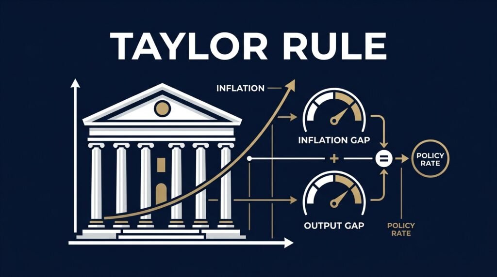
The Taylor Rule is the most influential quantitative guideline in modern macroeconomic policy. Formulated in 1993 by Stanford University economist John B. Taylor, this foundational framework provides a systematic formula for how a central bank should adjust its benchmark short-term nominal interest rate in response to two key economic variables: deviations of inflation from target and deviations of real economic output from its potential capacity.
Before John Taylor published his seminal paper, monetary policy was widely regarded outside central banking circles as an opaque, discretionary process. Taylor demonstrated that between 1987 and 1992, the policy choices of the Federal Reserve under Chairman Alan Greenspan could be modeled with remarkable precision using a straightforward mathematical equation. Today, central banks worldwide—including the Federal Reserve, the European Central Bank (ECB), the Bank of England, and the Reserve Bank of India—regularly consult Taylor-type policy rules as navigational benchmarks when evaluating interest rate decisions.
This comprehensive guide breaks down the theoretical foundations of the Taylor Rule, unpacks its mathematical formulation variable by variable, examines a step-by-step worked illustrative example, explores the pivotal Taylor Principle, and analyzes why modern policymakers treat the rule as an analytical compass rather than an autopilot.
1. Why Central Banks Use Policy Rules and Frameworks
To understand the importance of the Taylor Rule, one must first explore the foundational debate in monetary economics between discretion and rules. In a purely discretionary system, central bankers retain unconstrained freedom at each meeting to set policy rates based on immediate market sentiment, short-term data releases, or political pressures without forward commitment.
However, pioneering macroeconomic research by Nobel laureates Finn Kydland and Edward Prescott (1977), as well as Robert Barro and David Gordon (1983), demonstrated that pure discretion suffers from a critical flaw known as the time-inconsistency problem. If a central bank promises price stability but subsequently lowers interest rates to engineer an artificial short-term employment boom, rational workers and businesses quickly anticipate this incentive. Workers demand higher wages and firms raise prices, producing permanently higher inflation without any lasting gain in employment or real GDP.
A systematic monetary policy rule addresses this credibility challenge through three key channels:
- Anchoring Inflation Expectations: Committing to a transparent reaction function ensures households and financial markets know precisely how the central bank will react if inflation drifts above target.
- Reducing Market Volatility: Systematic policy dampens interest rate uncertainty, lowering risk premia across sovereign bond yields and commercial borrowing rates.
- Establishing Institutional Accountability: An explicit benchmark provides legislators and the public with an objective standard against which central bank choices can be evaluated.
2. The Original Taylor Rule Framework
In his 1993 study, “Discretion versus Policy Rules in Practice,” John B. Taylor showed that monetary policy operates with greatest stability when conducted according to a systematic strategy formally stated as an operational reaction function.
Analyzing historical data, Taylor demonstrated that Federal Reserve policy systematically tightened when inflation accelerated or economic output exceeded potential, and loosened when output contracted or inflation subsided.
3. The Mathematical Formula and Variables Explained
The classic 1993 specification of the Taylor Rule formula is written as:
it = r* + πt + 0.5(πt – π*) + 0.5(yt – y*)
To grasp the mechanics, consider each building block of the equation:
it — The Target Nominal Policy Interest Rate
The short-term nominal policy rate recommended by the rule for period t. In the United States, this corresponds to the federal funds rate; in the Eurozone, the main refinancing operations rate; and in India, the Reserve Bank of India’s policy repo rate.
r* — The Neutral (Equilibrium) Real Interest Rate
Known as r-star, this represents the theoretical real interest rate that neither stimulates nor restricts economic growth when the economy is at full employment with inflation at target. Taylor originally assumed r* = 2.0%, matching the long-term trend growth rate of U.S. real output per capita.
πt — The Current Inflation Rate
Prevailing annual inflation over the preceding four quarters, typically measured by the GDP deflator, headline Consumer Price Index (CPI), or Core Personal Consumption Expenditures (PCE) price index.
π* — The Central Bank’s Inflation Target
The official long-run inflation goal established by the central bank. In advanced economies (U.S., Eurozone, U.K., Japan), this target is typically 2.0%. In inflation-targeting emerging markets such as India, the statutory target is 4.0% (within a 2%–6% tolerance band).
(πt – π*) — The Inflation Gap
The gap between observed inflation and the target. When current inflation is 4.0% against a 2.0% target, the inflation gap is +2.0 percentage points, warranting monetary tightening. A negative gap calls for policy accommodation.
(yt – y*) — The Output Gap
The percentage deviation of actual real GDP (yt) from potential GDP (y*). A positive output gap indicates an overheating economy straining productive capacity, while a negative output gap reflects economic slack and underutilized labor and capital.
0.5 — The Response Coefficients (απ and αy)
The weights assigned to policy adjustments. A 1.0 percentage point rise in inflation adds 0.5 percentage points to the rate, while a 1.0% expansion above potential GDP adds an additional 0.5 percentage points.
4. Worked Illustrative Example: Step-by-Step Calculation
To examine formula mechanics, consider the following worked numerical scenario. (Note: This calculation is strictly an illustrative educational example to demonstrate formula mechanics and does not represent an actual central-bank recommendation or official policy forecast.)
Assumed Macroeconomic Baseline (Illustrative Scenario):
- Equilibrium neutral real rate (r*): 2.0%
- Central bank inflation target (π*): 2.0%
- Observed annual inflation rate (πt): 4.5%
- Estimated output gap (yt – y*): +1.0%
Step-by-Step Mathematical Calculation:
Step 1: Calculate the Inflation Gap
Inflation Gap = πt – π* = 4.5% – 2.0% = +2.5 percentage points
Step 2: Calculate the Output Gap
Output Gap = yt – y* = +1.0 percentage point
Step 3: Substitute Values into the Formula
it = r* + πt + 0.5(πt – π*) + 0.5(yt – y*)
it = 2.0% + 4.5% + 0.5(2.5%) + 0.5(1.0%)
Step 4: Solve for the Target Rate
Base Component (r* + πt) = 2.0% + 4.5% = 6.5%
Inflation Adjustment = 0.5 × 2.5% = +1.25%
Output Gap Adjustment = 0.5 × 1.0% = +0.50%
Recommended Nominal Rate (it) = 6.5% + 1.25% + 0.50% = 8.25%
In this illustrative scenario, the classic Taylor Rule prescribes an operational nominal policy rate of 8.25%. Because inflation exceeded target by 2.5 percentage points, the nominal policy rate was raised by 4.25 percentage points above the baseline neutral rate of 4.0% (2.0% r* + 2.0% target inflation), demonstrating the stabilizing power of systematic policy.
5. What Happens in Specific Macroeconomic Conditions?
What Happens When Inflation Rises Above Target? (The Taylor Principle)
The single most critical theoretical insight of the rule is the Taylor Principle: when inflation increases by 1.0 percentage point, the central bank must raise the nominal policy rate by more than 1.0 percentage point.
Regrouping the inflation terms from the equation yields:
it = r* – 0.5(π*) + 1.5(πt) + 0.5(yt – y*)
Notice the total coefficient on inflation is 1.5. Because 1.5 exceeds 1.0, an acceleration in inflation of 1.0 percentage point leads to a 1.5 percentage point increase in nominal rates. Consequently, the real interest rate (nominal rate minus inflation) increases by 0.5 percentage points:
Change in Real Rate = 1.5% – 1.0% = +0.5 percentage points
Higher real interest rates raise borrowing costs for mortgages and business loans, cooling aggregate demand and guiding inflation back to target. Conversely, if a central bank raises nominal rates by less than one-for-one (e.g., hiking by 0.7 percentage points when inflation rises by 1.0 point), real rates fall. Borrowing becomes cheaper in real terms, fueling credit expansion and causing an explosive inflationary spiral—a primary driver of the 1970s Great Inflation.
What Happens When Output Falls Below Potential?
During an economic recession, actual GDP falls below potential GDP, generating a negative output gap (e.g., yt – y* = -3.0%). In the formula, a negative gap subtracts from the policy rate (0.5 × -3.0% = -1.5 percentage points). Lower borrowing costs stimulate capital investment and consumer purchases, helping close the output gap.
6. Why the Taylor Rule Is Not an Automatic Policy-Setting Machine
Despite its mathematical rigor, no major central bank operates on a mechanical Taylor Rule autopilot. Policymakers treat the formula as an informative benchmark due to several real-world limitations:
A. Real-Time Data Revisions
Macroeconomic indicators are unobservable in real time. As economist Athanasios Orphanides demonstrated in 2001, GDP and output gap figures available at policy meetings are preliminary estimates subject to major subsequent revisions. Setting policy mechanically on unrevised data can cause central banks to overtighten into an economy that is already slowing down.
B. The Time-Varying Neutral Rate (r*)
Taylor assumed a constant r* of 2.0%. However, research by Laubach and Williams (2003) showed that neutral rates drift over time due to demographics, productivity shifts, and global savings trends. An incorrect estimate of r* causes a rule to prescribe policy that is persistently too tight or too loose.
C. Supply Shocks vs. Demand Shocks
The basic rule assumes demand shocks where inflation and output move together. During adverse supply shocks—such as oil price spikes or supply chain disruptions—inflation accelerates while output contracts (stagflation). The inflation gap demands rate hikes while the output gap demands rate cuts. A mathematical rule cannot weigh these trade-offs; human judgment and institutional credibility must decide the policy balance. For an examination of how external commodity shocks constrain policy, review our analysis on RBI’s Rate Turn: How Oil, the Fed and a Rupee Past 96 Cornered India’s Central Bank.
D. Financial Stability and the Effective Lower Bound
The classic formula omits financial stability, asset prices, and exchange rate volatility. During banking crises, preserving systemic liquidity takes precedence over domestic gap formulas. Furthermore, during severe recessions, the formula can prescribe negative rates, requiring central banks to deploy unconventional measures like quantitative easing. Prolonged structural imbalances can also entrench deflationary pressures, as documented in our study on why China Is Trapped in Deflation.
7. Different Versions of the Taylor Rule
To address practical shortcomings, economists have developed several alternative specifications:
- The Taylor 1999 Rule: Proposed by John Taylor in 1999, this variant doubled the output gap coefficient to 1.0 (it = r* + πt + 0.5(πt – π*) + 1.0(yt – y*)). By placing higher weight on economic slack, it prescribes sharper cuts during downturns, offering an improved fit during recoveries.
- The Inertial (Smoothing) Rule: Central banks prefer gradual rate adjustments. An inertial rule incorporates the lagged interest rate (it-1) with a smoothing weight (ρ ≈ 0.8): it = ρ·it-1 + (1 – ρ)·itTaylor, preventing abrupt bond market volatility.
- Forward-Looking Rules: Recognizing policy transmission lags of 12 to 18 months, Clarida, Galí, and Gertler (2000) formulated rules targeting projected future inflation (E[πt+k]) rather than backward-looking indicators.
8. Comparative Framework Summary
| Rule Variant | Formula / Specification | Key Strategic Emphasis | Best Suited For |
|---|---|---|---|
| Classic Taylor (1993) | it = r* + πt + 0.5(π – π*) + 0.5(y – y*) | Balanced, equal weights on inflation and output deviations | Normal business cycle conditions |
| Taylor (1999) | it = r* + πt + 0.5(π – π*) + 1.0(y – y*) | Higher sensitivity to output slack and unemployment | Severe recessions and post-crisis recoveries |
| Inertial Rule | it = ρ·it-1 + (1 – ρ)·itTaylor | Prevents abrupt policy volatility via gradual adjustments | Empirical central bank modeling |
| Forward-Looking Rule | it = r* + π* + β(E[πt+k] – π*) + γE[yt+k – y*] | Targets projected future inflation rather than backward data | Modern inflation-targeting frameworks |
9. Frequently Asked Questions (FAQ)
Is the Taylor Rule legally binding for the Federal Reserve?
No. The Federal Reserve operates under a statutory dual mandate from the U.S. Congress: maximum sustainable employment and price stability. While the Federal Open Market Committee (FOMC) reviews Taylor Rule paths in its briefing materials, decisions are made by committee vote and are not bound by formula.
What is the difference between percent and percentage points in the Taylor Rule?
Precision in units is essential in macroeconomic modeling. If inflation rises from 2.0% to 3.0%, it has increased by 1.0 percentage point in absolute terms, but by 50 percent in relative terms. The Taylor Principle specifically refers to percentage points: the central bank must raise nominal rates by more than 1.0 percentage point for every 1.0 percentage point rise in inflation.
How does the Taylor Rule apply to open economies and emerging markets?
In emerging markets like India, Brazil, or South Africa, central banks frequently augment the Taylor Rule with exchange rate terms and import price variables. Because currency depreciation transmits rapidly into domestic inflation and sovereign debt costs, central banks cannot focus exclusively on domestic gaps. For insights on sovereign debt interactions with global monetary frameworks, examine our explainer on How the IMF Actually Works.
10. Practical Takeaways for Students, Investors, and Observers
- A Transparent Benchmark, Not an Autopilot: The Taylor Rule provides a disciplined baseline for evaluating whether monetary policy is accommodative, restrictive, or neutral.
- The Taylor Principle Is Essential: The insight that real borrowing costs must rise when inflation accelerates remains the bedrock of central banking credibility.
- Parameter Sensitivity Matters: Policy recommendations depend heavily on unobservable parameters—especially neutral real rates (r*) and output gaps—meaning divergent economic assumptions yield divergent policy prescriptions.
- An Enduring Contribution: More than three decades after its introduction, the Taylor Rule remains the cornerstone of quantitative monetary economics and central bank communication.
References and Authoritative Literature
- Taylor, John B. (1993). “Discretion versus Policy Rules in Practice.” Carnegie-Rochester Conference Series on Public Policy, Vol. 39, pp. 195–214.
- Taylor, John B. (1999). “A Historical Analysis of Monetary Policy Rules.” In Monetary Policy Rules, National Bureau of Economic Research (NBER), University of Chicago Press.
- Kydland, Finn E., and Edward C. Prescott (1977). “Rules Rather than Discretion: The Inconsistency of Optimal Plans.” Journal of Political Economy, Vol. 85, No. 3, pp. 473–491.
- Orphanides, Athanasios (2001). “Monetary Policy Rules Based on Real-Time Data.” American Economic Review, Vol. 91, No. 4, pp. 964–985.
- Clarida, Richard, Jordi Galí, and Mark Gertler (2000). “Monetary Policy Rules and Macroeconomic Stability: Evidence and Some Theory.” Quarterly Journal of Economics, Vol. 115, No. 1, pp. 147–180.
- Laubach, Thomas, and John C. Williams (2003). “Measuring the Natural Rate of Interest.” Review of Economics and Statistics, Vol. 85, No. 4, pp. 1063–1070.
- Federal Reserve Board. “Monetary Policy Principles and Practice: Policy Rules.” Available via federalreserve.gov.
- Bank for International Settlements (BIS). “Monetary Policy Frameworks and Central Bank Balance Sheets.” Available via bis.org.