Table of Contents
- 1. What Is a Yield Curve Inversion?
- 2. Historical Track Record as a Recession Predictor
- 3. The Mathematical Mechanics: Term Premia & Expectations
- 4. Why Do Investors Buy Long-Term Bonds at Lower Yields?
- 5. Central Bank Dilemma: Inversion and Monetary Policy
- 6. Frequently Asked Questions (FAQ)
Among all forward-looking financial market metrics, few indicators command as much institutional respect as a yield curve inversion. In healthy macroeconomic environments, lending money for extended horizons demands higher compensation than short-term loans. When this foundational relationship flips—causing short-term government bond yields to trade above long-term yields—it signals severe economic distortion and has historically served as Wall Street’s most reliable recession forecasting mechanism.
Since 1955, an inverted U.S. Treasury yield curve has preceded every American recession, with only a single false positive in the mid-1960s. For central bankers, institutional asset allocators, and sovereign treasury desks, understanding why the curve inverts is not merely an academic exercise; it is an essential framework for assessing monetary policy restrictiveness, banking system liquidity, and macroeconomic credit contraction.
This comprehensive guide examines the mechanical structure of the term structure of interest rates, derives the mathematical forces driving inversions, evaluates the predictive accuracy of the 10-year minus 2-year and 10-year minus 3-month yield spreads, analyzes the role of the term premium, and explains why banking systems experience credit gridlock when the yield curve turns upside down.
1. The Mechanics of the Yield Curve: Normal vs. Inverted
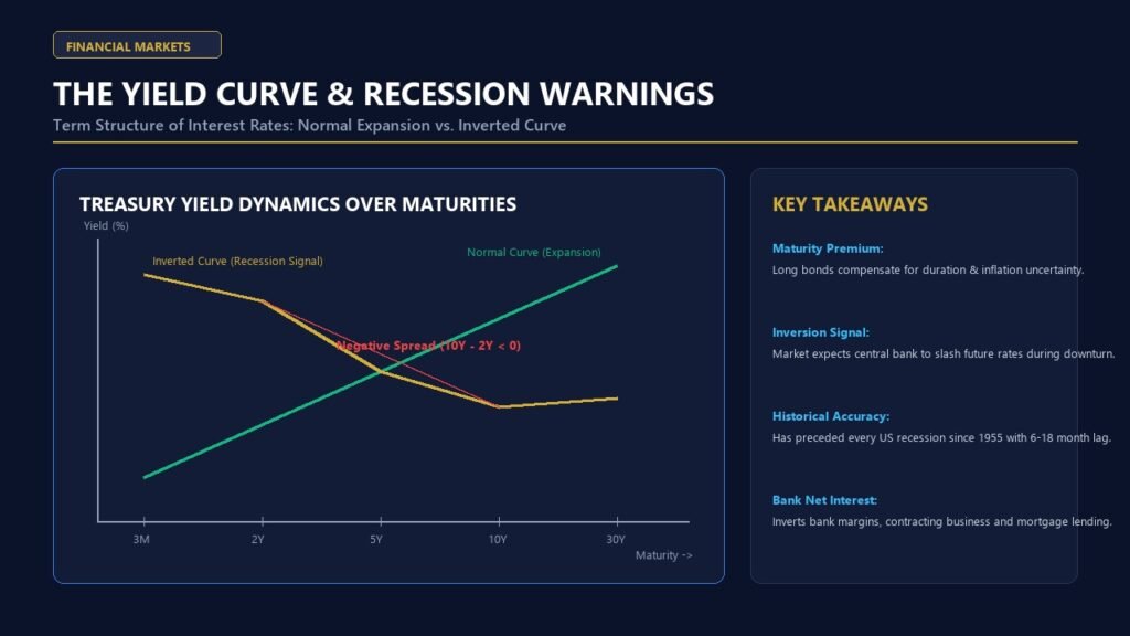
The yield curve is a graphical representation of the relationship between bond yields and bond maturities across sovereign debt of equal credit quality. Under standard macroeconomic conditions, the yield curve slopes upward from left to right. A 2-year government bond might yield 3.5%, while a 10-year bond yields 4.5%, and a 30-year bond yields 5.0%.
A. Why Normal Yield Curves Slope Upward
Three distinct theoretical mechanisms ensure that longer-term debt normally carries higher yields:
- Liquidity Preference: As formulated by John Maynard Keynes, investors inherently prefer liquidity. Locking capital into a 10-year or 30-year sovereign bond exposes the lender to capital losses if market interest rates rise. Investors demand a yield premium to sacrifice balance sheet liquidity.
- Duration Risk and Inflation Uncertainty: Over a multi-decade horizon, future purchasing power is vulnerable to unexpected inflationary shocks. Longer-dated bonds carry higher duration risk—meaning their prices are significantly more sensitive to interest rate fluctuations.
- The Term Premium: The excess return required by bondholders to compensate for the uncertainty of holding long-term debt rather than continuously rolling over short-term bills. The term premium ($TP_t$) is normally positive.
B. The Inversion Phenomenon
A yield curve inversion occurs when short-term yields surge above long-term yields. Under this condition, the yield spread—conventionally measured as the 10-Year Treasury Yield minus the 2-Year Treasury Yield ($y_{10} – y_2$) or the 10-Year Yield minus the 3-Month Treasury Bill Yield ($y_{10} – y_{3m}$)—drops below zero basis points.
When the 2-year Treasury trades at 5.00% while the 10-year Treasury trades at 4.25%, the spread is negative 75 basis points (-0.75 percentage points). The term structure is inverted, creating an anomalous market condition where long-term lenders accept lower annualized returns than overnight or short-term lenders.
2. Theoretical Foundations: The Expectations Hypothesis
To mathematically understand why the yield curve inverts, economists utilize the Pure Expectations Hypothesis of the Term Structure. According to this framework, a long-term bond yield represents the geometric average of expected future short-term interest rates over the life of the bond, plus a term premium:
$$(1 + y_{n,t})^n = \prod_{i=0}^{n-1} \left(1 + \mathbb{E}_t[r_{t+i}]\right) + TP_{n,t}$$
Approximated in linear terms:
$$y_{n,t} \approx \frac{1}{n} \sum_{i=0}^{n-1} \mathbb{E}_t[r_{t+i}] + TP_{n,t}$$
Where $y_{n,t}$ is the yield on an $n$-period sovereign bond at time $t$, $r_{t+i}$ is the short-term policy interest rate in period $t+i$, and $TP_{n,t}$ is the term premium.
When a central bank aggressively raises its benchmark policy rate to combat inflation (following frameworks like The Taylor Rule), the current short rate $r_t$ rises rapidly. Short-term yields (such as the 2-year yield) surge in direct alignment with central bank policy. However, institutional bond investors anticipate that these restrictive monetary conditions will inevitably slow economic growth, suppress inflation, and force the central bank to slash interest rates in years 3 through 10.
Because the 10-year yield reflects the average of these future expected rate cuts, it fails to keep pace with short-term yields. If the market anticipates aggressive future easing ($\mathbb{E}_t[r_{t+k}] \ll r_t$), the long-term yield drops below the short-term yield, enforcing an mathematical inversion.
3. The Dual Spreads: 10Y-2Y vs. 10Y-3M
In market commentary, two distinct Treasury spreads serve as primary recession benchmarks:
A. The 10-Year minus 2-Year Treasury Spread (T10Y2Y)
Popularized by financial media and institutional traders, the 10Y-2Y spread measures market sentiment regarding monetary policy trajectory over a medium-term horizon. Because both 2-year and 10-year notes are heavily traded coupon-bearing securities, this spread is liquid, reactive, and reflects market positioning months before monetary tightening cycles reach their terminal peak.
B. The 10-Year minus 3-Month Treasury Spread (T10Y3M)
Academic research conducted by the Federal Reserve Bank of New York—pioneered by economists Arturo Estrella and Frederic Mishkin—concludes that the 10-year minus 3-month spread is mathematically superior for formal recession probability modeling. The 3-month Treasury bill yield trades in lockstep with the immediate Federal Funds Rate, while the 10-year reflects long-term economic equilibrium. When the 3-month bill yield exceeds the 10-year note yield, monetary policy has achieved absolute restrictiveness relative to the economy’s neutral growth rate.
4. Why Yield Curve Inversions Cause Recessions
A vital question in monetary economics is whether a yield curve inversion is simply an optical thermometer that registers an impending downturn, or whether the inversion itself acts as an active catalyst that triggers economic contraction. Modern financial macroeconomics proves that it functions as both.
A. The Destruction of Banking Net Interest Margins (NIM)
Commercial banking relies on maturity transformation: banks borrow short (via customer deposits and repo markets) and lend long (through 30-year mortgages, corporate credit lines, and industrial term loans). When the yield curve slopes upward, this spread generates healthy Net Interest Margins (NIM).
When the curve inverts, short-term deposit funding costs rise above long-term asset yields. Commercial banks face severe margin compression. In response, banks aggressively tighten commercial lending standards, raise collateral hurdles, and reduce loan originations. This credit contraction starves small-and-medium enterprises (SMEs) of working capital, depressing private investment ($I$) and initiating layoffs.
B. Corporate Capital Expenditure Retrenchment
Corporate financial officers monitor sovereign term structures. An inverted curve signals that high current borrowing costs are temporary, while long-term consumer demand will soften. Rather than issuing debt at elevated short-term rates to fund factory expansions or equipment upgrades, corporations postpone capital expenditure (CapEx), wait for rate cuts, and build cash reserves, accelerating the downturn.
5. Historical Track Record and the Lag Dilemma
The historical reliability of the inverted yield curve is unmatched across modern macroeconomic forecasting:
- 1973 Oil Shock Recession: Curve inverted in June 1973; recession began in November 1973 (5-month lag).
- 1980 Volcker Disinflation: Curve inverted in August 1978; recession began in January 1980 (17-month lag).
- 1990 Savings and Loan Crisis: Curve inverted in January 1989; recession began in July 1990 (18-month lag).
- 2001 Dot-Com Crash: Curve inverted in February 2000; recession began in March 2001 (13-month lag).
- 2007–2008 Great Financial Crisis: Curve inverted in December 2005; recession began in December 2007 (24-month lag).
- 2020 COVID-19 Recession: Curve briefly inverted in August 2019; recession arrived in February 2020 (6-month lag).
Historical data reveals that the lag between the initial inversion and the official start of a recession averages between 12 and 18 months, occasionally extending past 24 months. Crucially, recessions historically do not begin when the curve is deeply inverted; they typically trigger when the yield curve un-inverts (steepens), as the central bank begins emergency interest rate cuts in response to rapid labor market deterioration.
6. Structural Complications: The Term Premium Distortion
In recent business cycles, central bank balance sheet policies—specifically Quantitative Easing (QE)—have introduced structural distortions into the term structure. By purchasing hundreds of billions of dollars in long-dated sovereign debt, central banks artificially suppressed the term premium ($TP$).
When the term premium is compressed to near zero or negative levels, a yield curve can invert with much smaller increases in short-term policy rates. Neoclassical economists, including former Federal Reserve Chairman Ben Bernanke, have noted that a low term premium can cause the yield curve to give a false or delayed signal. Nevertheless, empirical econometric studies by the Bank for International Settlements (BIS) and the International Monetary Fund (IMF) confirm that even in the post-QE era, yield curve inversions remain statistically significant harbingers of economic slowdowns.
7. Term Structure Regimes Compared
The table below summarizes the four distinct yield curve configurations, their underlying monetary drivers, and their economic implications:
| Yield Curve Shape | Spread Dynamics | Underlying Drivers | Macroeconomic Outlook |
|---|---|---|---|
| Normal (Upward Sloping) | Long yields significantly higher than short yields (+100 to +250 bps). | Economic expansion; healthy term premium; positive growth expectations. | Sustainable expansion; stable bank lending and corporate investment. |
| Flat Curve | Short and long yields roughly equal (0 to +25 bps). | Transition phase; central bank hiking rates; growth momentum cooling. | Cautionary signal; monetary tightening reaching restrictive territory. |
| Inverted Curve | Short yields higher than long yields (-25 to -150 bps). | Aggressive central bank rate hikes; market pricing in future economic contraction. | High recession probability within 12 to 24 months; bank credit tightening. |
| Bull Steepener (Un-inversion) | Short yields plunging faster than long yields as curve turns positive. | Emergency central bank rate cuts in response to rising unemployment. | Imminent or ongoing recession; labor market distress; credit stress. |
8. Frequently Asked Questions (FAQ)
What is the exact definition of a yield curve inversion?
A yield curve inversion occurs when the yields on short-term sovereign debt securities (such as 3-month bills or 2-year notes) rise above the yields on longer-term sovereign bonds (such as 10-year notes). This causes the spread between long-term and short-term yields to turn negative.
How long after a yield curve inversion does a recession begin?
Historically, the lag between initial inversion and the official National Bureau of Economic Research (NBER) recession declaration ranges from 6 to 24 months, with an average lag of roughly 14 months. The recession typically begins not during peak inversion, but when the curve rapidly steepens as central banks slash interest rates.
Why doesn’t an inverted yield curve guarantee a recession every single time?
While the historical correlation is exceptionally strong, macroeconomic shocks can alter outcomes. If productivity surges, supply bottlenecks resolve rapidly, or the term premium was abnormally depressed by central bank asset purchases, an economy may experience a “soft landing” or delayed slowdown rather than a formal technical recession.
How does an inverted yield curve affect everyday consumers?
An inverted curve causes banks to tighten credit card and mortgage lending standards. Consumers face higher borrowing costs on auto loans and home equity credit, while corporate hiring slows, increasing the risk of labor market retrenchment.
What is the difference between a Bear Flattener and a Bull Steepener?
A Bear Flattener occurs when short-term interest rates rise faster than long-term rates as a central bank aggressively hikes policy rates. A Bull Steepener occurs when short-term rates plunge rapidly because the central bank is cutting rates during an unfolding economic crisis.
9. Authoritative References & Sourcing
- Estrella, Arturo, and Frederic S. Mishkin (1998). “Predicting U.S. Recessions: Financial Variables as Leading Indicators”. Review of Economics and Statistics, 80(1), 45–61.
- Federal Reserve Bank of New York (2023). “The Yield Curve as a Leading Indicator: Historical Spreads and Recession Probabilities”.
- Keynes, John Maynard (1936). The General Theory of Employment, Interest and Money. London: Macmillan.
- Bank for International Settlements (BIS) (2022). “The Information Content of the Term Structure in a Changing Inflation Regime”. BIS Quarterly Review.
- International Monetary Fund (IMF) (2023). “Global Financial Stability Report: Navigating the High-for-Longer Interest Rate Cycle”.
- U.S. Department of the Treasury. Daily Treasury Par Yield Curve Rates.
- Federal Reserve Bank of St. Louis. FRED Economic Data: 10-Year Treasury Constant Maturity Minus 2-Year Treasury Constant Maturity (T10Y2Y).